Introduction • grates

Overview

The goal of grates is to make it easy to group dates across a range of different time intervals. It defines a collection of classes and associated methods that, together, formalise the concept of grouped dates and are intuitive to use. To assist in formatting plots of grates objects we also provides x-axis scales that can be used in conjunction with ggplot2 output. Currently implemented classes are:

grates_yearweek;
grates_epiweek;
grates_isoweek;
grates_period;
grates_yearmonth;
grates_yearquarter;
grates_year; and
grates_month

The underlying implementation for these objects build upon ideas of Davis Vaughan and the unreleased datea package as well as Zhian Kamvar and the aweek package.

Note that for brevity in the rest of the vignette, we will drop the grates_ prefix when discussing the underlying class.

grates objects

yearweek, epiweek and isoweek

yearweek objects are stored as the number of weeks (starting at 0L) from the date of the firstday nearest the Unix Epoch (1970-01-01). Put more simply, the number of seven day periods from:

1969-12-29 for firstday equal to 1 (Monday)
1969-12-30 for firstday equal to 2 (Tuesday)
1969-12-31 for firstday equal to 3 (Wednesday)
1970-01-01 for firstday equal to 4 (Thursday)
1970-01-02 for firstday equal to 5 (Friday)
1970-01-03 for firstday equal to 6 (Saturday)
1970-01-04 for firstday equal to 7 (Sunday)

They can be constructed directly from integers via the new_yearweek() function but it is generally easier to use the either the as_yearweek() coercion function or the yearweek() constructor. as_yearweek() takes two arguments; x, the vector (normally a Date or POSIXt) you wish to group, and firstday, the day of the week you wish your weeks to start on. yearweek() takes three arguments; year and week integer vectors and, again, a firstday value.

The epiweek class is similar to the yearweek class but, by definition, will always begin on a Sunday. They are stored as the integer number of weeks (again starting at 0L) since 1970-01-04 so internally are akin to grates_yearweek_sunday objects but with the benefit of slightly more efficient implementations for many of the associated methods.

Likewise, the isoweek class is similar to epiweek class but uses the ISO 8601 definition of a week that will always start on a Monday. Internally they are stored as the integer number of weeks since 1969-12-29.

library(grates)

# Choose some consecutive dates that begin on a Friday
first <- as.Date("2021-01-01")
weekdays(first)
#> [1] "Friday"
dates <- first + 0:9

# Below we use a Friday-week grouping
weeks <- as_yearweek(dates, firstday = 5L)
(dat <- data.frame(dates, weeks))
#>         dates    weeks
#> 1  2021-01-01 2021-W01
#> 2  2021-01-02 2021-W01
#> 3  2021-01-03 2021-W01
#> 4  2021-01-04 2021-W01
#> 5  2021-01-05 2021-W01
#> 6  2021-01-06 2021-W01
#> 7  2021-01-07 2021-W01
#> 8  2021-01-08 2021-W02
#> 9  2021-01-09 2021-W02
#> 10 2021-01-10 2021-W02

# we can also use the constructor function if we already have weeks and years
yearweek(year = c(2020L, 2021L), week = c(1L, 10L), firstday = 5L)
#> <grates_yearweek_friday[2]>
#> [1] "2020-W01" "2021-W10"

# epiweeks always start on a Sunday
(epiwk <- as_epiweek(Sys.Date()))
#> <grates_epiweek[1]>
#> [1] "2024-W47"

weekdays(as.Date(epiwk))
#> [1] "Sunday"

# isoweeks always start on a Sunday
(isowk <- as_isoweek(Sys.Date()))
#> <grates_isoweek[1]>
#> [1] "2024-W47"

weekdays(as.Date(isowk))
#> [1] "Monday"

By default plots (using ggplot2) will centre yearweek (epiweek / isoweek) labels:

library(ggplot2)

# use simulated linelist data from the outbreaks package
dat <- outbreaks::ebola_sim_clean
dat <- dat$linelist$date_of_infection

# calculate the total number for across each week
week_dat <- aggregate(
    list(cases = dat),
    by = list(week = as_epiweek(dat)),
    FUN = length
)

head(week_dat)
#>       week cases
#> 1 2014-W12     1
#> 2 2014-W15     1
#> 3 2014-W16     1
#> 4 2014-W17     3
#> 5 2014-W18     6
#> 6 2014-W19    16

# plot the output
(week_plot <-
    ggplot(week_dat, aes(week, cases)) +
    geom_col(width = 1, colour = "white") +
    theme_bw())

We can have non-centred date labels on the x_axis by utilising the associated scale_x_grates functions and explicitly specifying a format for the date labels:

week_plot + scale_x_grates_epiweek(format = "%Y-%m-%d")

Period

period objects are stored as the integer number, starting at 0L, of periods since the Unix Epoch (1970-01-01) and a specified offset. Here periods are taken to mean groupings of n consecutive days.

Like yearweek objects, a period object can be constructed directly via a call to new_period() but more easily via the as_period() coercion function. as_period() takes 3 arguments; x, the vector (normally a Date or POSIXt) you wish to group, n, the integer number of days you wish to group, and offset, the value you wish to start counting groups from relative to the Unix Epoch. For convenience, offset can be given as a date you want periods to be relative to (internally this date is converted to integer).

Note that storage and calculation purposes, offset is scaled relative to n. I.e. offset <- offset %% n and values of x stored relative to this scaled offset.

# calculate the total number for across 14 day periods with no offset.
# note - 0L is the default value for the offset but we specify it explicitly
# here for added clarity
period_dat <- aggregate(
    list(cases = dat),
    by = list(period = as_period(dat, n = 14L, offset = 0L)),
    FUN = length
)

head(period_dat)
#>                     period cases
#> 1 2014-03-13 to 2014-03-26     1
#> 2 2014-03-27 to 2014-04-09     1
#> 3 2014-04-10 to 2014-04-23     3
#> 4 2014-04-24 to 2014-05-07    19
#> 5 2014-05-08 to 2014-05-21    19
#> 6 2014-05-22 to 2014-06-04    30

ggplot(period_dat, aes(period, cases)) +
    geom_col(width = 1, colour = "white") +
    theme_bw() +
    theme(axis.text.x = element_text(angle = 45, hjust = 1)) +
    xlab("")

We can also use a date as an offset

dates <- as.Date("2020-01-03") + 0:9
offset <- as.Date("2020-01-01")
data.frame(dates, period = as_period(dates, n = 7L, offset = offset))
#>         dates                   period
#> 1  2020-01-03 2020-01-01 to 2020-01-07
#> 2  2020-01-04 2020-01-01 to 2020-01-07
#> 3  2020-01-05 2020-01-01 to 2020-01-07
#> 4  2020-01-06 2020-01-01 to 2020-01-07
#> 5  2020-01-07 2020-01-01 to 2020-01-07
#> 6  2020-01-08 2020-01-08 to 2020-01-14
#> 7  2020-01-09 2020-01-08 to 2020-01-14
#> 8  2020-01-10 2020-01-08 to 2020-01-14
#> 9  2020-01-11 2020-01-08 to 2020-01-14
#> 10 2020-01-12 2020-01-08 to 2020-01-14

yearmonth, yearquarter and year

yearmonth, yearquarter and year objects are stored as the integer number of months/quarters/years (starting at 0L) since the Unix Epoch (1970-01-01).

Similar to other grates objects we provide both coercion and construction functions.

(month_dat <- aggregate(
    list(cases = dat),
    by = list(month = as_yearmonth(dat)),
    FUN = length
))
#>       month cases
#> 1  2014-Mar     1
#> 2  2014-Apr     6
#> 3  2014-May    57
#> 4  2014-Jun    80
#> 5  2014-Jul   183
#> 6  2014-Aug   453
#> 7  2014-Sep   813
#> 8  2014-Oct   719
#> 9  2014-Nov   448
#> 10 2014-Dec   307
#> 11 2015-Jan   251
#> 12 2015-Feb   199
#> 13 2015-Mar   152
#> 14 2015-Apr    73

(month_plot <-
    ggplot(month_dat, aes(month, cases)) +
    geom_col(width = 1, colour = "white") +
    theme_bw() +
    theme(axis.text.x = element_text(angle = 45, hjust = 1)) +
    xlab(""))

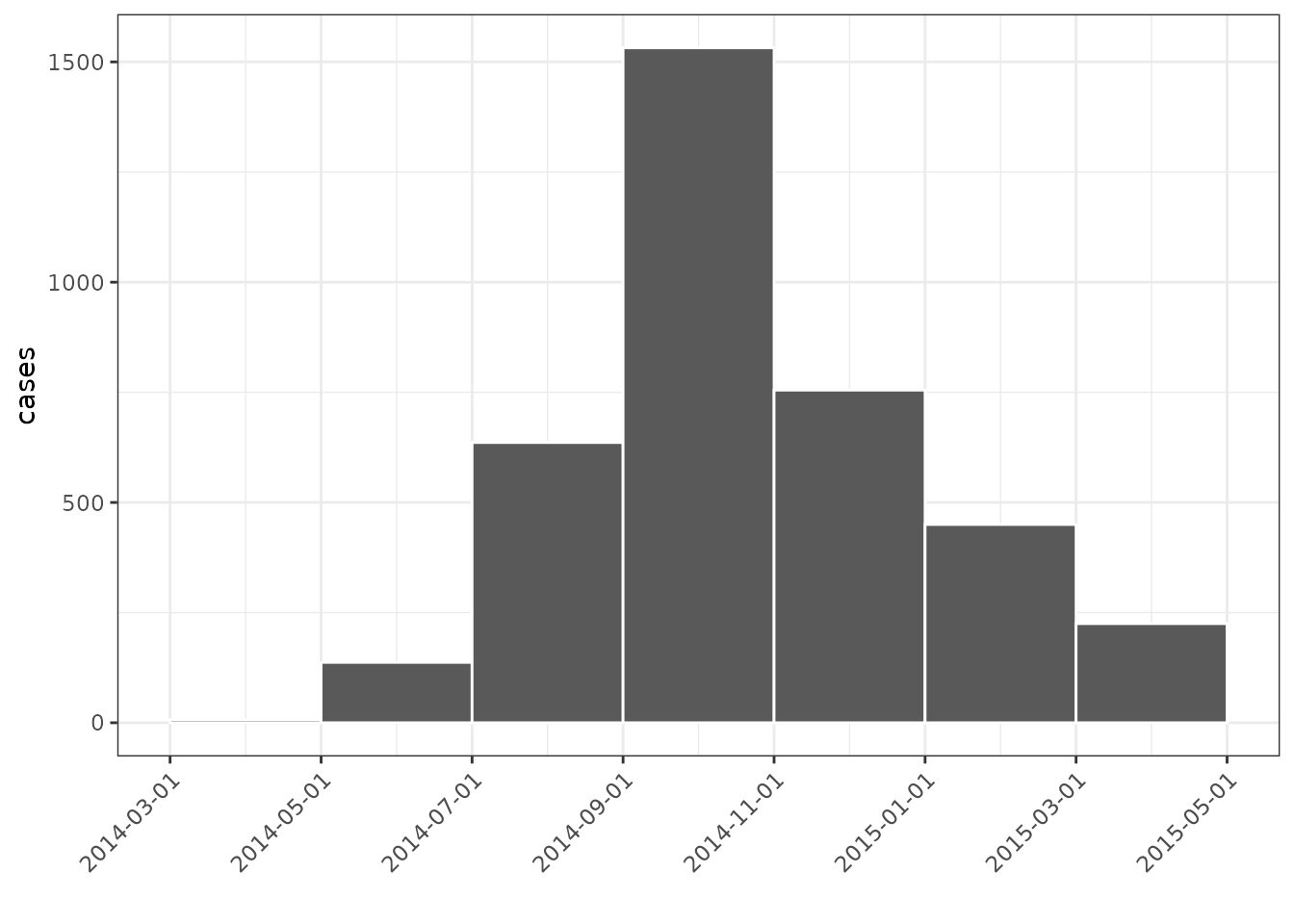
Again we can have non-centred date labels by applying the associated scale

month_plot + scale_x_grates_yearmonth(format = "%Y-%m-%d")

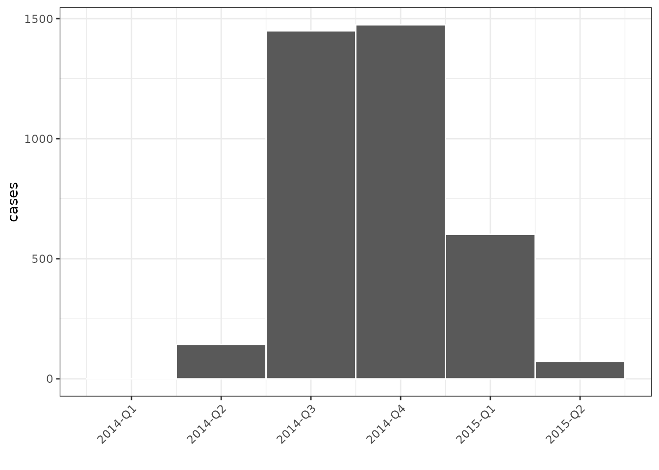
yearquarter works similarly

(quarter_dat <- aggregate(
    list(cases = dat),
    by = list(quarter = as_yearquarter(dat)),
    FUN = length
))
#>   quarter cases
#> 1 2014-Q1     1
#> 2 2014-Q2   143
#> 3 2014-Q3  1449
#> 4 2014-Q4  1474
#> 5 2015-Q1   602
#> 6 2015-Q2    73

ggplot(quarter_dat, aes(quarter, cases)) +
    geom_col(width = 1, colour = "white") +
    theme_bw() +
    theme(axis.text.x = element_text(angle = 45, hjust = 1)) +
    xlab("")

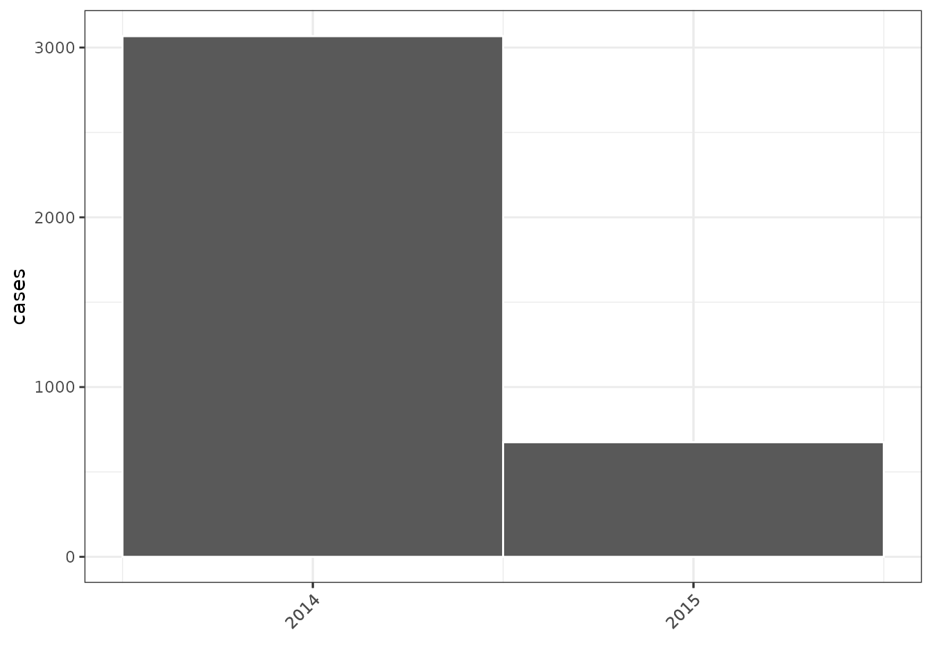
Bar chart of quarterly incidence (by date of infection) covering the time from 2014-Q1 to 2015-Q2 inclusive. The graph peaks over quarters 3 and 4 in 2014. Labels on the x-axis and of the form 'year-quarter' are centred on the corresponding bars.

As does year

(year_dat <- aggregate(
    list(cases = dat),
    by = list(year = as_year(dat)),
    length
))
#>   year cases
#> 1 2014  3067
#> 2 2015   675

ggplot(year_dat, aes(year, cases)) +
    geom_col(width = 1, colour = "white") +
    theme_bw() +
    theme(axis.text.x = element_text(angle = 45, hjust = 1)) +
    xlab("")

Bar chart of yearly incidence (by date of infection) for 2014 and 2015. There were lots more cases in 2014 compared to 2015 (Roughly speaking 3000 v 700).

# Construction functions can also be used
yearmonth(2022L, 11L)
#> <grates_yearmonth[1]>
#> [1] "2022-Nov"
yearquarter(2022L, 4L)
#> <grates_yearquarter[1]>
#> [1] "2022-Q4"
year(2022L)
#> <grates_year[1]>
#> [1] 2022

month

month objects are stored as the integer number of n-month groups (starting at 0L) since the Unix Epoch (1970-01-01). Here n-months is taken to mean a ‘grouping of n consecutive months’.

month objects can be constructed directly from integers via the new_month() function and through coercion via the as_month() function. as_period() takes two arguments; x, the vector (normally a Date or POSIXt) you wish to group and n, the integer number of months you wish to group.

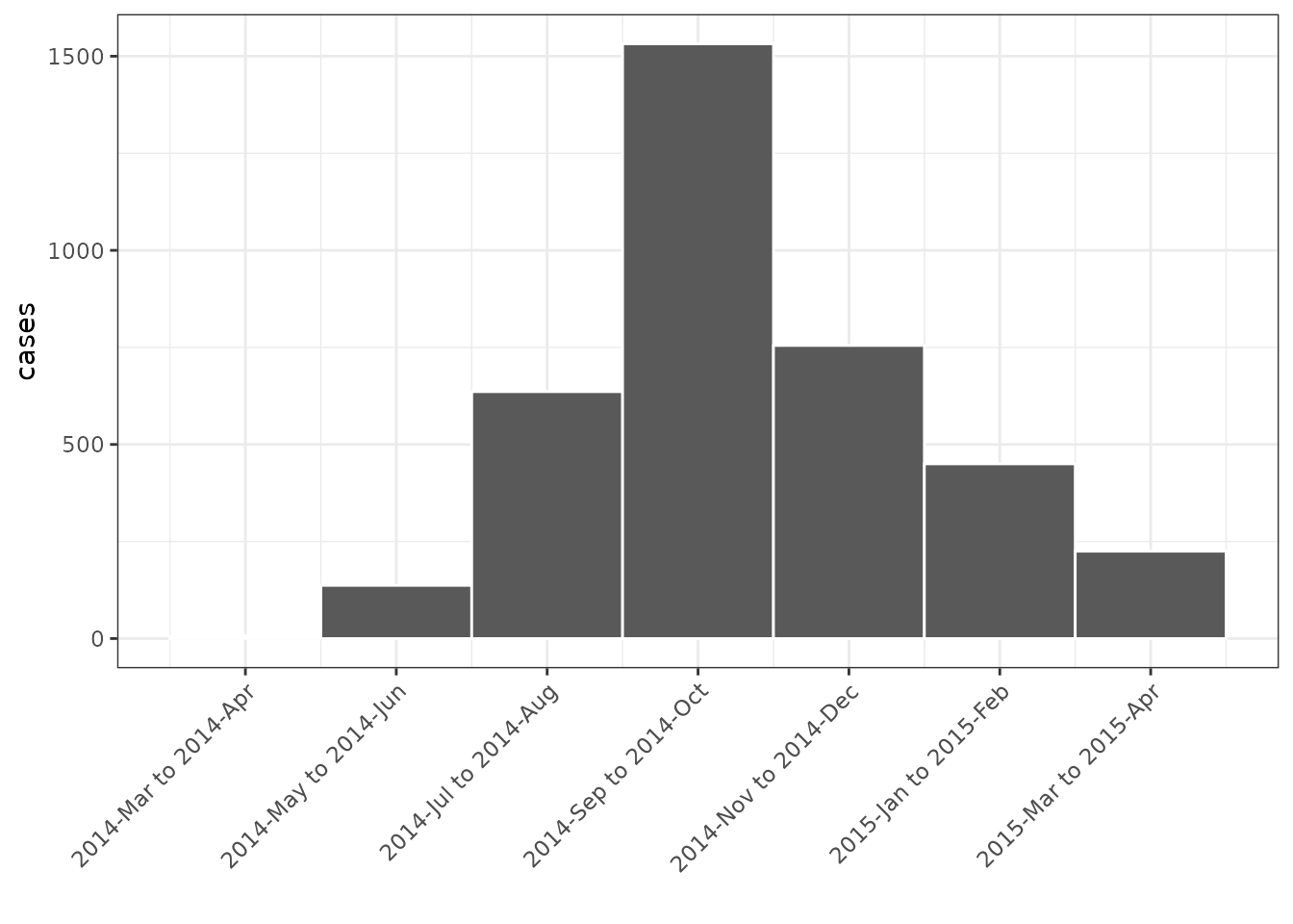
# calculate the bimonthly number of cases
(bimonth_dat <- aggregate(
    list(cases = dat),
    by = list(group = as_month(dat, n = 2L)),
    FUN = length
))
#>                  group cases
#> 1 2014-Mar to 2014-Apr     7
#> 2 2014-May to 2014-Jun   137
#> 3 2014-Jul to 2014-Aug   636
#> 4 2014-Sep to 2014-Oct  1532
#> 5 2014-Nov to 2014-Dec   755
#> 6 2015-Jan to 2015-Feb   450
#> 7 2015-Mar to 2015-Apr   225

# by default lower date bounds are used for the x axis
(bimonth_plot <-
    ggplot(bimonth_dat, aes(group, cases)) +
    geom_col(width = 1, colour = "white") +
    theme_bw() +
    theme(axis.text.x = element_text(angle = 45, hjust = 1)) +
    xlab(""))

Bar chart of bimonthly incidence (by date of infection) covering the time from March 2014 to April 2015 inclusive. The graph peaks around September/October 2014. Labels of the form 'year-month-day' are evenly spread along the x-axis aligned to the start of the corresponding bars.

Note that the default plotting behaviour of non-centred date labels is different to that of the yearweek, yearmonth, yearquarter and year scales where labels are centred by default. To obtain centred labels you must explicitly set the format to NULL in the scale:

bimonth_plot + scale_x_grates_month(format = NULL, n = 2L)

Bar chart of bimonthly incidence (by date of infection) covering the time from March 2014 to April 2015 inclusive. The graph peaks around September/October 2014. Labels of the form 'year-month to year-month' are evenly spread along the x-axis centred on the corresponding bars.

Methods and other functionality

For all grates objects we have added many methods and operations to ensure logical and consistent behaviour. The following sections utilise the unique epiweeks from the earlier example:

weeks <- week_dat$week

Accessing boundary values and checking contents

Some times it is useful to access both the starting dates covered by grates objects as well as the end dates. To this end we provide functions date_start() and date_end().

To find out whether a grate object spans a particular date we provide a %during% function.

dat <- weeks[1:5]
data.frame(
    week = dat,
    start = date_start(dat),
    end = date_end(dat),
    contains.2014.04.14 = as.Date("2014-04-14") %during% dat
)
#>       week      start        end contains.2014.04.14
#> 1 2014-W12 2014-03-16 2014-03-22               FALSE
#> 2 2014-W15 2014-04-06 2014-04-12               FALSE
#> 3 2014-W16 2014-04-13 2014-04-19                TRUE
#> 4 2014-W17 2014-04-20 2014-04-26               FALSE
#> 5 2014-W18 2014-04-27 2014-05-03               FALSE

Conversion of grate objects back to dates is analogous to date_start().

identical(as.Date(weeks), date_start(weeks))
#> [1] TRUE

min, max, range and sequences

# min, max and range
(minw <- min(weeks))
#> <grates_epiweek[1]>
#> [1] "2014-W12"
(maxw <- max(weeks))
#> <grates_epiweek[1]>
#> [1] "2015-W17"
(rangew <- range(weeks))
#> <grates_epiweek[2]>
#> [1] "2014-W12" "2015-W17"

# seq method works if both `from` and `to` are epiweeks
seq(from = minw, to = maxw, by = 6L)
#> <grates_epiweek[10]>
#>  [1] "2014-W12" "2014-W18" "2014-W24" "2014-W30" "2014-W36" "2014-W42"
#>  [7] "2014-W48" "2015-W01" "2015-W07" "2015-W13"

# but will error informatively if `to` is a different class
try(seq(from = minw, to = 999, by = 6L))
#> Error in seq.grates_epiweek(from = minw, to = 999, by = 6L) : 
#>   `to` must be a <grates_epiweek> object of length 1.

Addition and subtraction

Addition (subtraction) of whole numbers will add (subtract) the corresponding number of weeks to (from) the object

dat <- head(week_dat)
(dat <- transform(dat, plus4 = week + 4L, minus4 = week - 4L))
#>       week cases    plus4   minus4
#> 1 2014-W12     1 2014-W16 2014-W08
#> 2 2014-W15     1 2014-W19 2014-W11
#> 3 2014-W16     1 2014-W20 2014-W12
#> 4 2014-W17     3 2014-W21 2014-W13
#> 5 2014-W18     6 2014-W22 2014-W14
#> 6 2014-W19    16 2014-W23 2014-W15

Addition of two yearweek objects will error as the intention is unclear.

try(transform(dat, willerror = week + week))
#> Error in Ops.grates_epiweek(week, week) : 
#>   Cannot add <grates_epiweek> objects to each other.

Subtraction of two yearweek objects gives the difference in weeks between them

transform(dat, difference = plus4 - minus4)
#>       week cases    plus4   minus4 difference
#> 1 2014-W12     1 2014-W16 2014-W08    8 weeks
#> 2 2014-W15     1 2014-W19 2014-W11    8 weeks
#> 3 2014-W16     1 2014-W20 2014-W12    8 weeks
#> 4 2014-W17     3 2014-W21 2014-W13    8 weeks
#> 5 2014-W18     6 2014-W22 2014-W14    8 weeks
#> 6 2014-W19    16 2014-W23 2014-W15    8 weeks

epiweek objects can be combined with themselves but not other classes (assuming an epiweek object is the first entry).

c(minw, maxw)
#> <grates_epiweek[2]>
#> [1] "2014-W12" "2015-W17"
identical(c(minw, maxw), rangew)
#> [1] TRUE

try(c(minw, 1L))
#> Error in c.grates_epiweek(minw, 1L) : 
#>   Unable to combine <grates_epiweek> objects with other classes.