Help pages

get_date_index_name(x, ...)

## Default S3 method:
get_date_index_name(x, ...)

## S3 method for class 'incidence2'
get_date_index_name(x, ...)

get_dates_name(x, ...)

get_count_variable_name(x, ...)

## Default S3 method:
get_count_variable_name(x, ...)

## S3 method for class 'incidence2'
get_count_variable_name(x, ...)

get_count_value_name(x, ...)

## Default S3 method:
get_count_value_name(x, ...)

## S3 method for class 'incidence2'
get_count_value_name(x, ...)

get_group_names(x, ...)

## Default S3 method:
get_group_names(x, ...)

## S3 method for class 'incidence2'
get_group_names(x, ...)

get_date_index(x, ...)

## Default S3 method:
get_date_index(x, ...)

## S3 method for class 'incidence2'
get_date_index(x, ...)

get_dates(x, ...)

get_count_variable(x, ...)

## Default S3 method:
get_count_variable(x, ...)

## S3 method for class 'incidence2'
get_count_variable(x, ...)

get_count_value(x, ...)

## Default S3 method:
get_count_value(x, ...)

## S3 method for class 'incidence2'
get_count_value(x, ...)

get_groups(x, ...)

## Default S3 method:
get_groups(x, ...)

## S3 method for class 'incidence2'
get_groups(x, ...)

Arguments

`x`	An R object.
`...`	Not currently used.

Value

get_date_index_name(): The name of the date_index variable of x.
get_dates_name(): Alias for get_date_index_name().
get_count_variable_name(): The name of the count variable of x.
get_count_value_name(): The name of the count value of x.
get_group_names(): The name(s) of the group variable(s) of x.
get_date_index(): The date_index variable of x.
get_dates(): Alias for get_date_index().
get_count_variable(): The count variable of x.
get_count_value(): The count value of x.
get_groups(): List of the group variable(s) of x.

Examples

if (requireNamespace("outbreaks", quietly = TRUE)) {
    data(ebola_sim_clean, package = "outbreaks")
    dat <- ebola_sim_clean$linelist
    i <- incidence(
        dat,
        date_index = "date_of_onset",
        groups = c("gender", "hospital")
    )
    get_count_variable_name(i)
    get_group_names(i)
    get_dates_name(i)
}

#> [1] "date_index"

Coerce to and from an incidence object

Description

Generic for coercion to an <incidence2> object.

Usage

as_incidence(x, ...)

## Default S3 method:
as_incidence(x, ...)

## S3 method for class 'incidence2'
as_incidence(x, ...)

## S3 method for class 'incidence2'
as.data.frame(x, row.names, optional, ...)

## S3 method for class 'incidence2'
as.data.table(x, keep.rownames, ...)

## S3 method for class 'incidence2'
as_tibble(x, ..., .rows, .name_repair, rownames)

Arguments

`x`	An R object.
`...`	Additional arguments to be passed to or from other methods.
`row.names`	Not used.
`optional`	Not used.
`keep.rownames`	Not used.
`.rows`	The number of rows, useful to create a 0-column tibble or just as an additional check.
`.name_repair`	Treatment of problematic column names: `"minimal"`: No name repair or checks, beyond basic existence, `"unique"`: Make sure names are unique and not empty, `"check_unique"`: (default value), no name repair, but check they are `unique`, `"universal"`: Make the names `unique` and syntactic a function: apply custom name repair (e.g., `.name_repair = make.names` for names in the style of base R). A purrr-style anonymous function, see `rlang::as_function()` This argument is passed on as `repair` to `vctrs::vec_as_names()`. See there for more details on these terms and the strategies used to enforce them.
`rownames`	How to treat existing row names of a data frame or matrix: `NULL`: remove row names. This is the default. `NA`: keep row names. A string: the name of a new column. Existing rownames are transferred into this column and the `row.names` attribute is deleted. No name repair is applied to the new column name, even if `x` already contains a column of that name. Use `as_tibble(rownames_to_column(...))` to safeguard against this case. Read more in rownames.

Value

An object of the desired type with additional attributes dropped.

Examples

if (requireNamespace("outbreaks", quietly = TRUE)) {
    data(ebola_sim_clean, package = "outbreaks")
    dat <- ebola_sim_clean$linelist
    x <- incidence(dat, "date_of_onset")
    as.data.frame(dat)
    as.data.table(x)
    as_tibble(x)
}

#> # A tibble: 367 × 3
#>    date_index count_variable count
#>    <date>     <chr>          <int>
#>  1 2014-04-07 date_of_onset      1
#>  2 2014-04-15 date_of_onset      1
#>  3 2014-04-21 date_of_onset      2
#>  4 2014-04-25 date_of_onset      1
#>  5 2014-04-26 date_of_onset      1
#>  6 2014-04-27 date_of_onset      1
#>  7 2014-05-01 date_of_onset      2
#>  8 2014-05-03 date_of_onset      1
#>  9 2014-05-04 date_of_onset      1
#> 10 2014-05-05 date_of_onset      1
#> # ℹ 357 more rows

Bootstrap incidence time series

Description

This function can be used to bootstrap incidence2 objects. Bootstrapping is done by sampling with replacement the original input dates.

Usage

bootstrap_incidence(x, randomise_groups = FALSE)

Arguments

x

An incidence2 object.

randomise_groups

bool.

Should groups be randomised as well in the resampling procedure; respective group sizes will be preserved, but this can be used to remove any group-specific temporal dynamics.

If FALSE (default), data are resampled within groups.

Details

As original data are not stored in incidence2 objects, the bootstrapping is achieved by multinomial sampling of date bins weighted by their relative incidence.

Value

An incidence2 object.

Author(s)

Thibaut Jombart, Tim Taylor

Examples

if (requireNamespace("outbreaks", quietly = TRUE)) {
    data(fluH7N9_china_2013, package = "outbreaks")
    i <- incidence(
        fluH7N9_china_2013,
        date_index = "date_of_onset",
        groups = "gender"
   )
   bootstrap_incidence(i)
}

#> # incidence:  67 x 4
#> # count vars: date_of_onset
#> # groups:     gender
#>    date_index gender count_variable count
#>  * <date>     <fct>  <chr>          <int>
#>  1 2013-02-19 m      date_of_onset      0
#>  2 2013-02-27 m      date_of_onset      1
#>  3 2013-03-07 m      date_of_onset      1
#>  4 2013-03-08 m      date_of_onset      0
#>  5 2013-03-09 f      date_of_onset      0
#>  6 2013-03-13 f      date_of_onset      0
#>  7 2013-03-17 m      date_of_onset      1
#>  8 2013-03-19 f      date_of_onset      5
#>  9 2013-03-20 f      date_of_onset      2
#> 10 2013-03-20 m      date_of_onset      1
#> # ℹ 57 more rows

Complete dates for all group combinations

Description

This function ensures that an incidence object has the same range of dates for each grouping. By default missing counts will be filled with 0L.

Usage

complete_dates(x, expand = TRUE, fill = 0L, by = 1L, allow_POSIXct = FALSE)

Arguments

`x`	`<incidence2>` object.
`expand`	`logical`. Should a range of dates from the minimum to maximum value of the date index also be created. If `expand` is TRUE (default) then complete_dates will attempt to use `function(x) seq(min(x), max(x), by = 1)` to generate a complete sequence of dates.
`fill`	`numeric`. The value to replace missing counts by. Defaults to `0L`.
`by`	`Defunct`. Ignored.
`allow_POSIXct`	`logical`. Should this function work with POSIXct dates? Defaults to `FALSE`.

Value

An incidence2 object.

Examples

x <- data.frame(
    dates = Sys.Date() + c(1,3,4),
    groups = c("grp1","grp2", "grp1"),
    counts = 1:3
)

i <- incidence(x, date_index = "dates", groups = "groups", counts = "counts")
complete_dates(i)

#> # incidence:  8 x 4
#> # count vars: counts
#> # groups:     groups
#>   date_index groups count_variable count
#>   <date>     <chr>  <fct>          <int>
#> 1 2025-03-12 grp1   counts             1
#> 2 2025-03-12 grp2   counts             0
#> 3 2025-03-13 grp1   counts             0
#> 4 2025-03-13 grp2   counts             0
#> 5 2025-03-14 grp1   counts             0
#> 6 2025-03-14 grp2   counts             2
#> 7 2025-03-15 grp1   counts             3
#> 8 2025-03-15 grp2   counts             0

Regional data for COVID-19 cases in the UK

Description

A dataset containing the daily time-series of cases, tests, hospitalisations, and deaths for UK.

Usage

covidregionaldataUK

Format

A data frame with 6370 rows and 26 variables:

date: the date that the counts were reported (YYYY-MM-DD)
region: the region name
region_code: the region code
cases_new: new reported cases for that day
cases_total: total reported cases up to and including that day
deaths_new: new reported deaths for that day
deaths_total: total reported deaths up to and including that day
recovered_new: new reported recoveries for that day
recovered_total: total reported coveries up to and including that day
hosp_new: new reported hospitalisations for that day
hosp_total: total reported hospitalisations up to and including that day (note this is cumulative total of new reported, not total currently in hospital).
tested_new: tests for that day
tested_total: total tests completed up to and including that day

Details

Extracted using the covidregionaldata package on 2021-06-03.

Source

https://CRAN.R-project.org/package=covidregionaldata

Compute cumulative 'incidence'

Description

cumulate() computes the cumulative incidence over time for an incidence2 object.

Usage

cumulate(x)

Arguments

`x`	incidence2 object.

Examples

dat <- data.frame(
  dates = as.integer(c(0,1,2,2,3,5,7)),
  groups = factor(c(1, 2, 3, 3, 3, 3, 1))
)

i <- incidence(dat, date_index = "dates", groups = "groups")
cumulate(i)

#> # incidence:  6 x 4
#> # count vars: dates
#> # groups:     groups
#>   date_index groups count_variable cumulative_count
#> *      <int> <fct>  <chr>                     <int>
#> 1          0 1      dates                         1
#> 2          7 1      dates                         2
#> 3          1 2      dates                         1
#> 4          2 3      dates                         2
#> 5          3 3      dates                         3
#> 6          5 3      dates                         4

dplyr and tidyr verbs

Description

dplyr and tidyr methods that implicitly account for the inherent grouping structure of incidence2 objects.

Usage

## S3 method for class 'incidence2'
mutate(
  .data,
  ...,
  .by,
  .keep = c("all", "used", "unused", "none"),
  .before = NULL,
  .after = NULL
)

## S3 method for class 'incidence2'
nest(.data, ..., .by, .key, .names_sep)

## S3 method for class 'incidence2'
summarise(.data, ..., .by, .groups)

Arguments

`.data`	An incidence2 object.
`...`	Only used by `mutate()` and `summarise()` and, in which case, passed to underlying dplyr function.
`.by`	Not used as grouping structure implicit.
`.keep`	Control which columns from `.data` are retained in the output. Grouping columns and columns created by `...` are always kept. `"all"` retains all columns from `.data`. This is the default. `"used"` retains only the columns used in `...` to create new columns. This is useful for checking your work, as it displays inputs and outputs side-by-side. `"unused"` retains only the columns not used in `...` to create new columns. This is useful if you generate new columns, but no longer need the columns used to generate them. `"none"` doesn't retain any extra columns from `.data`. Only the grouping variables and columns created by `...` are kept.
`.before`, `.after`	<`tidy-select`> Optionally, control where new columns should appear (the default is to add to the right hand side). See `relocate()` for more details.
`.key`	The name of the resulting nested column. Only applicable when `...` isn't specified, i.e. in the case of `df %>% nest(.by = x)`. If `NULL`, then `"data"` will be used by default.
`.names_sep`	Not used.
`.groups`	Not used.

Value

For mutate() a modified incidence2 object if the necessary invariants are preserved, otherwise a tibble.
For nest() a nested tibble with rows corresponding to the count variable and (optionally) group columns of the input object.
For summarise a tibble with rows corresponding to the underlying groupings. The columns are a combination of the grouping keys and the summary expressions provided.

Examples

if (requireNamespace("outbreaks", quietly = TRUE) && requireNamespace("ggplot2", quietly = TRUE)) {
    data(ebola_sim_clean, package = "outbreaks")
    x <- subset(ebola_sim_clean$linelist, !is.na(hospital))
    dat <- incidence_(x, date_of_onset, hospital, interval = "isoweek")

    mutate(dat, ave = data.table::frollmean(count, n = 3L, align = "right")) |>
        plot(border_colour = "white", angle = 45) +
        ggplot2::geom_line(ggplot2::aes(x = date_index, y = ave))

    nest(dat)

    summarise(dat, model = list(glm(count ~ date_index, family = "poisson")))
}

#> # A tibble: 5 × 3
#>   count_variable hospital                                     model 
#>   <chr>          <fct>                                        <list>
#> 1 date_of_onset  Military Hospital                            <glm> 
#> 2 date_of_onset  Connaught Hospital                           <glm> 
#> 3 date_of_onset  other                                        <glm> 
#> 4 date_of_onset  Princess Christian Maternity Hospital (PCMH) <glm> 
#> 5 date_of_onset  Rokupa Hospital                              <glm>

Estimate the peak date of an incidence curve

Description

This function can be used to estimate the peak of an epidemic curve using bootstrapped samples of the available data.

Usage

estimate_peak(x, n = 100L, alpha = 0.05, first_only = TRUE, progress = TRUE)

Arguments

`x`	An incidence2 object.
`n`	`integer`. The number of bootstrap datasets to be generated; defaults to 100. `[double]` vectors will be converted via `as.integer(n)`.
`alpha`	`numeric`. The type 1 error chosen for the confidence interval; defaults to 0.05.
`first_only`	`bool`. Should only the first peak (by date) be kept. Defaults to `TRUE`.
`progress`	`bool`. Should a progress bar be displayed (default = TRUE)

Details

Input dates are resampled with replacement to form bootstrapped datasets; the peak is reported for each, resulting in a distribution of peak times. When there are ties for peak incidence, only the first date is reported.

Note that the bootstrapping approach used for estimating the peak time makes the following assumptions:

the total number of event is known (no uncertainty on total incidence)
dates with no events (zero incidence) will never be in bootstrapped datasets
the reporting is assumed to be constant over time, i.e. every case is equally likely to be reported

Value

A data frame with the the following columns:

observed_date: the date of peak incidence of the original dataset.
observed_count: the peak incidence of the original dataset.
estimated: the median peak time of the bootstrap datasets.
lower_ci/upper_ci: the confidence interval based on bootstrap datasets.
bootstrap_peaks: a nested tibble containing the the peak times of the bootstrapped datasets.

Author(s)

Thibaut Jombart and Tim Taylor, with inputs on caveats from Michael Höhle.

Examples

if (requireNamespace("outbreaks", quietly = TRUE)) {

  # load data and create incidence
  data(fluH7N9_china_2013, package = "outbreaks")
  i <- incidence(fluH7N9_china_2013, date_index = "date_of_onset")

  # find 95% CI for peak time using bootstrap
  estimate_peak(i)
}

#> # A tibble: 1 × 7
#>   count_variable observed_peak observed_count bootstrap_peaks lower_ci  
#>   <chr>          <date>                 <int> <list>          <date>    
#> 1 date_of_onset  2013-04-03                 7 <df [100 × 1]>  2013-03-28
#> # ℹ 2 more variables: median <date>, upper_ci <date>

Compute the incidence of events

Description

incidence() calculates the incidence of different events across specified time periods and groupings. incidence_() does the same but with support for tidy-select semantics in some of its arguments.

Usage

incidence(
  x,
  date_index,
  groups = NULL,
  counts = NULL,
  count_names_to = "count_variable",
  count_values_to = "count",
  date_names_to = "date_index",
  rm_na_dates = TRUE,
  interval = NULL,
  offset = NULL,
  complete_dates = FALSE,
  fill = 0L,
  ...
)

incidence_(
  x,
  date_index,
  groups = NULL,
  counts = NULL,
  count_names_to = "count_variable",
  count_values_to = "count",
  date_names_to = "date_index",
  rm_na_dates = TRUE,
  interval = NULL,
  offset = NULL,
  complete_dates = FALSE,
  ...
)

Arguments

`x`	A data frame object representing a linelist or pre-aggregated dataset.
`date_index`	`character` for `incidence()` or tidy-select for `incidence_()`. The time index(es) of the given data. This should be the name(s) corresponding to the desired date column(s) in x. A named vector can be used for convenient relabelling of the resultant output. Multiple indices only make sense when `x` is a linelist.
`groups`	`character` for `incidence()` or tidy-select for `incidence_()`. An optional vector giving the names of the groups of observations for which incidence should be grouped. A named vector can be used for convenient relabelling of the resultant output.
`counts`	`character` for `incidence()` or tidy-select for `incidence_()`. The count variables of the given data. If NULL (default) the data is taken to be a linelist of individual observations. A named vector can be used for convenient relabelling of the resultant output.
`count_names_to`	`character`. The column to create which will store the `counts` column names provided that `counts` is not NULL.
`count_values_to`	`character`. The name of the column to store the resultant count values in.
`date_names_to`	`character`. The name of the column to store the date variables in.
`rm_na_dates`	`bool`. Should `NA` dates be removed prior to aggregation?
`interval`	An optional scalar integer or string indicating the (fixed) size of the desired time interval you wish to use for for computing the incidence. Defaults to NULL in which case the date_index columns are left unchanged. Numeric values are coerced to integer and treated as a number of days to group. Text strings can be one of: `* day or daily * week(s) or weekly * epiweek(s) * isoweek(s) * month(s) or monthly * yearmonth(s) * quarter(s) or quarterly * yearquarter(s) * year(s) or yearly` More details can be found in the "Interval specification" section.
`offset`	Only applicable when `interval` is not NULL. An optional scalar integer or date indicating the value you wish to start counting periods from relative to the Unix Epoch: Default value of NULL corresponds to 0L. For other integer values this is stored scaled by `n` (`offset <- as.integer(offset) %% n`). For date values this is first converted to an integer offset (`offset <- floor(as.numeric(offset))`) and then scaled via `n` as above.
`complete_dates`	`bool`. Should the resulting object have the same range of dates for each grouping. Missing counts will be filled with `0L` unless the `fill` argument is provided (and this value will take precedence). Will attempt to use `function(x) seq(min(x), max(x), by = 1)` on the resultant date_index column to generate a complete sequence of dates. More flexible completion is possible by using the `complete_dates()` function.
`fill`	`numeric`. Only applicable when `complete_dates = TRUE`. The value to replace missing counts caused by completing dates. If unset then will default to `0L`.
`...`	Not currently used.

Details

incidence2 objects are a sub class of data frame with some additional invariants. That is, an incidence2 object must:

have one column representing the date index (this does not need to be a date object but must have an inherent ordering over time);
have one column representing the count variable (i.e. what is being counted) and one variable representing the associated count;
have zero or more columns representing groups;
not have duplicated rows with regards to the date and group variables.

Value

A tibble with subclass incidence2.

Interval specification

Where interval is specified, incidence(), predominantly uses the grates package to generate appropriate date groupings. The grouping used depends on the value of interval. This can be specified as either an integer value or a string corresponding to one of the classes:

integer values: <grates_period> object, grouped by the specified number of days.
day, daily: <Date> objects.
week(s), weekly, isoweek: <grates_isoweek> objects.
epiweek(s): <grates_epiweek> objects.
month(s), monthly, yearmonth: <grates_yearmonth> objects.
quarter(s), quarterly, yearquarter: <grates_yearquarter> objects.
year(s) and yearly: <grates_year> objects.

For "day" or "daily" interval, we provide a thin wrapper around as.Date() that ensures the underlying data are whole numbers and that time zones are respected. Note that additional arguments are not forwarded to as.Date() so for greater flexibility users are advised to modifying your input prior to calling incidence().

Examples

if (requireNamespace("outbreaks", quietly = TRUE)) {
    data(ebola_sim_clean, package = "outbreaks")
    dat <- ebola_sim_clean$linelist
    incidence(dat, "date_of_onset")
    incidence_(dat, date_of_onset)
    incidence(dat, "date_of_onset", groups = c("gender", "hospital"))
    incidence_(dat, date_of_onset, groups = c(gender, hospital))
}

#> # incidence:  2,535 x 5
#> # count vars: date_of_onset
#> # groups:     gender, hospital
#>    date_index gender hospital                               count_variable count
#>    <date>     <fct>  <fct>                                  <chr>          <int>
#>  1 2014-04-07 f      Military Hospital                      date_of_onset      1
#>  2 2014-04-15 m      Connaught Hospital                     date_of_onset      1
#>  3 2014-04-21 f      other                                  date_of_onset      1
#>  4 2014-04-21 m      other                                  date_of_onset      1
#>  5 2014-04-25 f      <NA>                                   date_of_onset      1
#>  6 2014-04-26 f      other                                  date_of_onset      1
#>  7 2014-04-27 f      <NA>                                   date_of_onset      1
#>  8 2014-05-01 f      Princess Christian Maternity Hospital… date_of_onset      1
#>  9 2014-05-01 f      Rokupa Hospital                        date_of_onset      1
#> 10 2014-05-03 f      Connaught Hospital                     date_of_onset      1
#> # ℹ 2,525 more rows

Functions now defunct in package incidence2

Description

These functions are now defunct.

Usage

new_incidence(
  x,
  date,
  groups = NULL,
  counts,
  measurements = NULL,
  validate = TRUE
)

validate_incidence(x)

build_incidence(
  x,
  date_index,
  groups = NULL,
  counts = NULL,
  na_as_group = TRUE,
  FUN = identity,
  args = list()
)

get_n(x)

get_interval(x, ...)

get_timespan(x, ...)

facet_plot(x, ...)

Keep first, last and peak occurences

Description

keep_first() and keep_last() keep the first and last n rows to occur for each grouping when in ascending date order. keep_peaks() keeps the rows with the maximum count value for each group. first_peak() is a convenience wrapper around keep_peaks() with the first_only argument set to TRUE.

Usage

keep_first(x, n, complete_dates = TRUE, ...)

keep_last(x, n, complete_dates = TRUE, ...)

keep_peaks(x, complete_dates = TRUE, first_only = FALSE, ...)

first_peak(x, complete_dates = TRUE, ...)

Arguments

`x`	incidence2 object.
`n`	`integer`. Number of entries to keep. `double` vectors will be converted via `as.integer(n)`.
`complete_dates`	`bool`. Should `complete_dates()` be called on the data prior to keeping the first entries. Defaults to TRUE.
`...`	Other arguments passed to `complete_dates()`.
`first_only`	`bool`. Should only the first peak (by date) be kept. Defaults to `TRUE`.

Value

incidence2 object with the chosen entries.

Examples

if (requireNamespace("outbreaks", quietly = TRUE)) {
    data(ebola_sim_clean, package = "outbreaks")
    dat <- ebola_sim_clean$linelist
    inci <- incidence(dat, "date_of_onset")
    keep_first(inci, 3)
    keep_last(inci, 3)
}

#> # incidence:  3 x 3
#> # count vars: date_of_onset
#>   date_index count_variable count
#>   <date>     <chr>          <int>
#> 1 2015-04-28 date_of_onset      8
#> 2 2015-04-29 date_of_onset      2
#> 3 2015-04-30 date_of_onset      2

Color palettes used in incidence

Description

These functions are color palettes used in incidence. The palettes come from https://personal.sron.nl/~pault/#sec:qualitative and exclude grey, which is reserved for missing data.

Usage

vibrant(n)

muted(n)

Arguments

`n`	`integer`. Number of colours. `double` vectors will be converted via `as.integer(n)`.

Examples

vibrant(5)

#> [1] "#0077BB" "#33BBEE" "#009988" "#EE7733" "#CC3311"

muted(10)

#> Using more colors (10) than this palette can handle (9); some colors will be interpolated.

#>  [1] "#332288" "#7EB9E2" "#53B1AB" "#228855" "#5C8933" "#B7AF51" "#D7AA77"
#>  [8] "#BC566F" "#8B255C" "#AA4499"

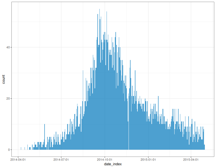
Plot an incidence object

Description

plot() can be used to provide a bar plot of an incidence object. Due to the complexities with automating plotting it is some what experimental in nature and it may be better to use ggplot2 directly.

Usage

## S3 method for class 'incidence2'
plot(
  x,
  y,
  width = 1,
  colour_palette = vibrant,
  border_colour = NA,
  na_colour = "grey",
  alpha = 0.7,
  fill = NULL,
  legend = c("right", "left", "bottom", "top", "none"),
  title = NULL,
  angle = 0,
  size = NULL,
  nrow = NULL,
  n_breaks = 6L,
  show_cases = FALSE,
  ...
)

Arguments

`x`	incidence2 object.
`y`	Not used. Required for compatibility with the `plot()` generic.
`width`	`numeric`. Value between 0 and 1 indicating the relative size of the bars to the interval. Default 1.
`colour_palette`	`function`. The color palette to be used for the different count variables. Defaults to `vibrant` (see `?palettes`).
`border_colour`	`character`. The color to be used for the borders of the bars. Use `NA` (default) for invisible borders.
`na_colour`	`character`. The colour to plot `NA` values in graphs. Defaults to `grey`.
`alpha`	`numeric`. The alpha level for color transparency, with 1 being fully opaque and 0 fully transparent Defaults to 0.7.
`fill`	`character`. Which variable to colour plots by. Must be a `group` or `count` variable and will mean that variable is not used for facetting. If NULL no distinction if made for plot colours.
`legend`	`character`. Position of legend in plot. Only applied if `fill` is not NULL. One of "right" (default), "left", "bottom", "top" or "none".
`title`	`character`. Optional title for the graph.
`angle`	`numeric`. Rotation angle for text.
`size`	`numeric`. text size in pts.
`nrow`	`integer`. Number of rows used for facetting if there are group variables present and just one count in the incidence object. Numeric values are coerced to integer via `as.integer()`.
`n_breaks`	`integer`. Approximate number of breaks calculated using `scales::breaks_pretty()`. Numeric values are coerced to integer via `as.integer()`. Default 6L.
`show_cases`	`logical`. if `TRUE`, then each observation will be shown individually in a square format. Normally only used for outbreaks with a small number of cases. Defaults to `FALSE`.
`...`	Not currently used.

Details

Faceting will occur automatically if either grouping variables or multiple counts are present.
If there are multiple count variables, each count will occupy a different row of the resulting plot.
Utilises ggplot2 so this must be installed to use.

Value

A ggplot2::ggplot() object.

Examples

if (requireNamespace("outbreaks", quietly = TRUE) && requireNamespace("ggplot2", quietly = TRUE)) {
    data(ebola_sim_clean, package = "outbreaks")
    dat <- ebola_sim_clean$linelist

    inci <- incidence(dat, date_index = "date_of_onset", groups = "hospital")
    plot(inci, angle = 45)

    inci2 <- regroup(inci)
    plot(inci2)
}

A plot recorded by xfun::record()

Objects exported from other packages

Description

These objects are imported from other packages. Follow the links below to see their documentation.

data.table: as.data.table
dplyr: mutate, select, summarise
tibble: as_tibble
tidyr: nest, unnest, unpack

Regroup 'incidence' objects

Description

This function regroups an incidence2 object across the specified groups. The resulting incidence2 object will contains counts aggregated over the specified groups. The only difference between regroup() and regroup_() is that the latter is built on top of tidy-select semantics for the group input.

Usage

regroup(x, groups = NULL)

regroup_(x, groups = NULL)

Arguments

x

<incidence2> object.

groups

character for regroup() or tidy-select for regroup_().

The groups to sum over.

If NULL (default) then the function returns the corresponding object with no groupings.

Examples

if (requireNamespace("outbreaks", quietly = TRUE)) {
    data(ebola_sim_clean, package = "outbreaks")
    dat <- ebola_sim_clean$linelist
    i <- incidence(
        dat,
        date_index = "date_of_onset",
        groups = c("gender", "hospital")
    )
    regroup(i)
    regroup_(i)
    regroup(i, "hospital")
    regroup_(i, hospital)
}

#> # incidence:  1,635 x 4
#> # count vars: date_of_onset
#> # groups:     hospital
#>    date_index hospital                                     count_variable count
#>    <date>     <fct>                                        <chr>          <int>
#>  1 2014-04-07 Military Hospital                            date_of_onset      1
#>  2 2014-04-15 Connaught Hospital                           date_of_onset      1
#>  3 2014-04-21 other                                        date_of_onset      2
#>  4 2014-04-25 <NA>                                         date_of_onset      1
#>  5 2014-04-26 other                                        date_of_onset      1
#>  6 2014-04-27 <NA>                                         date_of_onset      1
#>  7 2014-05-01 Princess Christian Maternity Hospital (PCMH) date_of_onset      1
#>  8 2014-05-01 Rokupa Hospital                              date_of_onset      1
#>  9 2014-05-03 Connaught Hospital                           date_of_onset      1
#> 10 2014-05-04 <NA>                                         date_of_onset      1
#> # ℹ 1,625 more rows

Divide an incidence2 object in to it's implicit groupings

Description

Split divides and incidence2 object in to it's underlying groupings (count variable and optionally groups).

Usage

## S3 method for class 'incidence2'
split(x, f, drop, ...)

Arguments

`x`	An incidence2 object.
`f`	Not used. Present only for generic compatibility.
`drop`	Not used. Present only for generic compatibility.
`...`	Not used. Present only for generic compatibility.

Value

A list of tibbles contained the split data. This list also has a "key" attribute which is a tibble with rows corresponding to the grouping of each split.

Examples

if (requireNamespace("outbreaks", quietly = TRUE)) {
    data(ebola_sim_clean, package = "outbreaks")
    ebola_sim_clean$linelist |>
        subset(!is.na(hospital)) |>
        incidence_(date_of_onset, hospital, interval = "isoweek") |>
        split()
}

#> [[1]]
#> # A tibble: 53 × 4
#>    date_index hospital          count_variable count
#>    <isowk>    <fct>             <chr>          <int>
#>  1 2014-W15   Military Hospital date_of_onset      1
#>  2 2014-W19   Military Hospital date_of_onset      5
#>  3 2014-W20   Military Hospital date_of_onset      4
#>  4 2014-W21   Military Hospital date_of_onset      3
#>  5 2014-W22   Military Hospital date_of_onset      2
#>  6 2014-W23   Military Hospital date_of_onset      2
#>  7 2014-W24   Military Hospital date_of_onset      4
#>  8 2014-W25   Military Hospital date_of_onset      1
#>  9 2014-W26   Military Hospital date_of_onset      3
#> 10 2014-W27   Military Hospital date_of_onset      4
#> # ℹ 43 more rows
#> 
#> [[2]]
#> # A tibble: 54 × 4
#>    date_index hospital           count_variable count
#>    <isowk>    <fct>              <chr>          <int>
#>  1 2014-W16   Connaught Hospital date_of_onset      1
#>  2 2014-W18   Connaught Hospital date_of_onset      1
#>  3 2014-W19   Connaught Hospital date_of_onset      3
#>  4 2014-W20   Connaught Hospital date_of_onset      2
#>  5 2014-W21   Connaught Hospital date_of_onset      5
#>  6 2014-W22   Connaught Hospital date_of_onset      4
#>  7 2014-W23   Connaught Hospital date_of_onset      6
#>  8 2014-W24   Connaught Hospital date_of_onset      6
#>  9 2014-W25   Connaught Hospital date_of_onset     12
#> 10 2014-W26   Connaught Hospital date_of_onset      8
#> # ℹ 44 more rows
#> 
#> [[3]]
#> # A tibble: 53 × 4
#>    date_index hospital count_variable count
#>    <isowk>    <fct>    <chr>          <int>
#>  1 2014-W17   other    date_of_onset      3
#>  2 2014-W19   other    date_of_onset      1
#>  3 2014-W20   other    date_of_onset      5
#>  4 2014-W21   other    date_of_onset      1
#>  5 2014-W22   other    date_of_onset      3
#>  6 2014-W23   other    date_of_onset      3
#>  7 2014-W24   other    date_of_onset      2
#>  8 2014-W25   other    date_of_onset      5
#>  9 2014-W26   other    date_of_onset      2
#> 10 2014-W27   other    date_of_onset      9
#> # ℹ 43 more rows
#> 
#> [[4]]
#> # A tibble: 50 × 4
#>    date_index hospital                                     count_variable count
#>    <isowk>    <fct>                                        <chr>          <int>
#>  1 2014-W18   Princess Christian Maternity Hospital (PCMH) date_of_onset      1
#>  2 2014-W19   Princess Christian Maternity Hospital (PCMH) date_of_onset      1
#>  3 2014-W20   Princess Christian Maternity Hospital (PCMH) date_of_onset      1
#>  4 2014-W21   Princess Christian Maternity Hospital (PCMH) date_of_onset      2
#>  5 2014-W22   Princess Christian Maternity Hospital (PCMH) date_of_onset      4
#>  6 2014-W25   Princess Christian Maternity Hospital (PCMH) date_of_onset      3
#>  7 2014-W27   Princess Christian Maternity Hospital (PCMH) date_of_onset      4
#>  8 2014-W28   Princess Christian Maternity Hospital (PCMH) date_of_onset      2
#>  9 2014-W29   Princess Christian Maternity Hospital (PCMH) date_of_onset      7
#> 10 2014-W30   Princess Christian Maternity Hospital (PCMH) date_of_onset      5
#> # ℹ 40 more rows
#> 
#> [[5]]
#> # A tibble: 51 × 4
#>    date_index hospital        count_variable count
#>    <isowk>    <fct>           <chr>          <int>
#>  1 2014-W18   Rokupa Hospital date_of_onset      1
#>  2 2014-W19   Rokupa Hospital date_of_onset      1
#>  3 2014-W20   Rokupa Hospital date_of_onset      1
#>  4 2014-W22   Rokupa Hospital date_of_onset      2
#>  5 2014-W23   Rokupa Hospital date_of_onset      2
#>  6 2014-W24   Rokupa Hospital date_of_onset      1
#>  7 2014-W25   Rokupa Hospital date_of_onset      1
#>  8 2014-W27   Rokupa Hospital date_of_onset      1
#>  9 2014-W28   Rokupa Hospital date_of_onset      5
#> 10 2014-W29   Rokupa Hospital date_of_onset      4
#> # ℹ 41 more rows
#> 
#> attr(,"key")
#> # A tibble: 5 × 2
#>   count_variable hospital                                    
#>   <chr>          <fct>                                       
#> 1 date_of_onset  Military Hospital                           
#> 2 date_of_onset  Connaught Hospital                          
#> 3 date_of_onset  other                                       
#> 4 date_of_onset  Princess Christian Maternity Hospital (PCMH)
#> 5 date_of_onset  Rokupa Hospital

Summary of an incidence object

Description

Summary of an incidence object

Usage

## S3 method for class 'incidence2'
summary(object, ...)

Arguments

`object`	An incidence2 object.
`...`	Not used.

Value

object (invisibly).

Examples

data(ebola_sim_clean, package = "outbreaks")
dat <- ebola_sim_clean$linelist
inci <- incidence(dat, "date_of_onset", groups = c("gender", "hospital"))
summary(inci)

#> From:          2014-04-07
#> To:            2015-04-30
#> Groups:        gender, hospital
#> 
#> Total observations:
#> # A data frame: 12 × 4
#>    gender hospital                                     count_variable count
#>    <fct>  <fct>                                        <chr>          <int>
#>  1 f      Military Hospital                            date_of_onset    439
#>  2 m      Connaught Hospital                           date_of_onset    848
#>  3 f      other                                        date_of_onset    437
#>  4 m      other                                        date_of_onset    439
#>  5 f      <NA>                                         date_of_onset    739
#>  6 f      Princess Christian Maternity Hospital (PCMH) date_of_onset    220
#>  7 f      Rokupa Hospital                              date_of_onset    210
#>  8 f      Connaught Hospital                           date_of_onset    889
#>  9 m      Rokupa Hospital                              date_of_onset    241
#> 10 m      Military Hospital                            date_of_onset    450
#> 11 m      Princess Christian Maternity Hospital (PCMH) date_of_onset    200
#> 12 m      <NA>                                         date_of_onset    717

Help pages

Access various elements of an incidence object

Description

Usage

Arguments

Value

Examples

Coerce to and from an incidence object

Description

Usage

Arguments

Value

Examples

Bootstrap incidence time series

Description

Usage

Arguments

Details

Value

Author(s)

Examples

Complete dates for all group combinations

Description

Usage

Arguments

Value

Examples

Regional data for COVID-19 cases in the UK

Description

Usage

Format

Details

Source

Compute cumulative 'incidence'

Description

Usage

Arguments

Examples

dplyr and tidyr verbs

Description

Usage

Arguments

Value

See Also

Examples

Estimate the peak date of an incidence curve

Description

Usage

Arguments

Details

Value

Author(s)

See Also

Examples

Compute the incidence of events

Description

Usage

Arguments

Details

Value

Interval specification

See Also

Examples

Functions now defunct in package incidence2

Description

Usage

Keep first, last and peak occurences

Description

Usage

Arguments

Value

Examples

Color palettes used in incidence

Description

Usage

Arguments

Examples

Plot an incidence object

Description

Usage